Tutorial

This tutorial walks through a complete optimisation run: wrapping a blackbox function in an Objective, configuring the search, executing the run, and reading the reproducibility record it leaves behind.

Setup

git clone https://github.com/AlxndrSchroeder/actgpr.git
cd actgpr
poetry install

Step 1: give it an Objective

actgpr minimises anything exposing an evaluate method that takes the coordinates of one input point, one argument per input, and returns that point’s one output as a float. It is called once per input point, never with several points at once. actgpr never checks whether that object is a particular type, only that the method exists (duck typing). Which of the two ways below to use depends on what you’re wrapping.

Wrapping a plain function

Use ObjectiveFn, a convenience that turns a plain function, taking one float per input and returning one float, into an Objective. This is the right choice when your blackbox is already a simple function:

from actgpr import ObjectiveFn

def my_blackbox(x: float) -> float:
    """Stand-in for a simulation or experiment."""
    return (x - 1) ** 2

objective = ObjectiveFn(my_blackbox)

objective.evaluate takes one input point and returns its output:

objective.evaluate(0.0)   # 1.0
objective.evaluate(3.0)   # 4.0

A function of several inputs simply takes several arguments, and evaluate passes the coordinates through in the same order:

def my_blackbox_3d(x1: float, x2: float, x3: float) -> float:
    return (x1 - 0.5) ** 2 + (x2 + 1.0) ** 2 + 0.2 * (x3 - 2.0) ** 2

ObjectiveFn(my_blackbox_3d).evaluate(0.5, -1.0, 2.0)   # 0.0, one 3D point

Several arguments are therefore always the coordinates of one point. To evaluate several points, call evaluate once for each.

Errors raised inside your function propagate unchanged, so you can handle them by their original type.

Simulating experimental noise

A real experiment’s readings are noisy, while an analytic stand-in like my_blackbox above is not. Pass jitter to add independent Gaussian noise to each evaluation, simulating that sensor/measurement noise:

noisy_objective = ObjectiveFn(my_blackbox, jitter=0.1)

If you use jitter, set the surrogate’s noise (Step 2) to match. jitter is a standard deviation, noise is a variance, so pass noise=jitter**2:

run = OptimisationRun.with_training(
    objective=noisy_objective,
    surrogate=GPyTorchSurrogate(),
    search_bounds=(-3.0, 5.0),
    initial_train_x=[-3.0, 5.0],
    max_iterations=20,
    ei_threshold=0.001,
    noise=0.1**2,   # matches noisy_objective's jitter=0.1
)

Without this, the GP starts out assuming noise’s default of near-zero observation noise (1e-4) and will overfit to what is actually random jitter, mistaking noise for real structure in the objective. with_training still tunes noise further from there, so passing a realistic starting value just gets it started in the right place.

The jitter noise comes from a generator the ObjectiveFn owns, seeded with 25 by default, so a jittered run reproduces without you seeding anything and the noise does not disturb the global torch RNG. Pass a different seed for a different noise sequence:

ObjectiveFn(my_blackbox, jitter=0.1, seed=7)

Wrapping your own simulation

If you already have a simulation or experiment of your own, meaning not just a bare function but something with setup, configuration, or state involved, write your own class with an evaluate() method instead of reaching for ObjectiveFn. This is the more natural fit for anything beyond a single pure function call, and it requires no base class or registration:

class MySimulation:
    """Wraps an existing simulation as an actgpr Objective."""

    def __init__(self, config):
        self.config = config  # e.g. simulation setup, fixed parameters

    def evaluate(self, pressure: float, temperature: float) -> float:
        # Called once per input point, with one argument per input.
        return self._run_simulation(pressure, temperature)

    def _run_simulation(self, pressure: float, temperature: float) -> float:
        ...  # launch your simulation at this input point, return its output

objective = MySimulation(config=...)

OptimisationRun only ever calls objective.evaluate(...). It never checks whether objective is an ObjectiveFn, so a class like this one works exactly the same way.

That is deliberate, not an oversight: it is what lets you plug in a simulation of your own without adapting it to actgpr. The interface is declared as a typing.Protocol (actgpr.objective_fn.Objective), so a type checker accepts your class too, even though it inherits nothing and registers nowhere.

Step 2: configure the run

Three decisions matter most:

search_bounds

One closed interval (lo, hi) per input, in which the algorithm searches for the minimum. The number of intervals is the number of inputs of the problem. A single (lo, hi) means one input. The blackbox is never evaluated outside these intervals.

max_iterations

The budget cap: the maximum number of active optimisation iterations (GPR fit cycles).

ei_threshold

The convergence threshold: the run stops early once the best achievable Expected Improvement falls below this value, meaning the surrogate sees nothing left to gain.

You also choose a fit mode:

• OptimisationRun.with_training(...) re-tunes the GP hyperparameters (lengthscale, outputscale, noise) at every iteration using Adam (GPyTorch’s torch.optim.Adam integration), a gradient-descent variant that maximises the marginal log likelihood, meaning how plausible the observed training data is under the GP. Use this when you do not know good hyperparameters, which is the usual case.

• OptimisationRun.without_training(...) keeps hyperparameters fixed at the values you pass. Use this for controlled comparisons or when good values are already known.

from actgpr import GPyTorchSurrogate, OptimisationRun

run = OptimisationRun.with_training(
    objective=objective,
    surrogate=GPyTorchSurrogate(),
    search_bounds=(-3.0, 5.0),   # interval in which the minimum is searched
    initial_train_x=[-3.0, 5.0],  # points where we start looking for the minimum
    max_iterations=20,
    ei_threshold=0.001,
    run_dir="results",            # write the MRR record
)

More than one input

Nothing else changes for several inputs. Give one (lo, hi) pair per input, and write each starting point as a row with one coordinate per input:

run = OptimisationRun.with_training(
    objective=ObjectiveFn(my_blackbox_3d),
    surrogate=GPyTorchSurrogate(),
    search_bounds=[(-2.0, 2.0), (-3.0, 1.0), (0.0, 5.0)],  # x1, x2, x3
    initial_train_x=[[-1.0, 0.0, 1.0], [1.5, -2.5, 4.0]],  # two 3D points
    max_iterations=20,
    ei_threshold=1e-4,
    run_dir="results",
)

Everything has to agree with the number of intervals, and a mismatch fails before the Objective is ever called:

• A flat initial_train_x=[0.0, 1.0] is accepted with one input (two 1D points) but rejected with two inputs, since it could mean one 2D point or two 1D points. Write [[0.0, 1.0]].

• A starting point with the wrong number of coordinates raises a ValueError saying how many were expected.

• A starting point outside its own (lo, hi) raises a ValueError naming the point and the input. The Objective is never evaluated outside the search bounds, so a starting point outside them would be the one exception.

• without_training takes lengthscale as one value for all inputs, or as a list with one value per input, e.g. lengthscale=[0.5, 3.0]. Inputs usually vary on different scales, which is why the GP keeps one lengthscale per input; with_training tunes each of them.

With one input, the acquisition function scores an evenly spaced grid of n_candidates points. With more inputs a grid is unaffordable (500 per input is 125 million points in 3D), so the candidates are drawn from a scrambled Sobol sequence instead, which covers the space evenly. The sequence is seeded with 25 and the seed is recorded in config.json, so a multi-input run reproduces exactly. n_candidates is then spread across all inputs, so raise it for problems with many inputs, but not without limit: prediction cost grows faster than linearly with it (on a laptop about 0.04 s per stage at 2048 candidates and 4 s at 16384, with two stages per iteration), so a few thousand is a sensible ceiling.

How precise is it with several inputs?

Less precise than with one input, and it is worth knowing why before trusting a result.

Each iteration picks its next point in stages: a coarse pass over the whole search space, then a refinement pass that re-searches a box around the best point so far. The box follows the candidate spacing, and candidates thin out quickly as inputs are added. With the default candidate count:

Inputs	Candidates (default)	Per axis	Box after 1st refinement	After 2nd
1	500	500	0.8 %	not used
2	4000	63.2	6.4 %	0.41 %
3	4000	15.9	26.9 %	7.2 %

This is why a run with more than one input refines twice while a single input refines once. In one dimension the first box is already 0.8 % of the axis, and a second pass would shrink it to the spacing between the points of a converged run, which risks evaluating the same point twice. Pass refinement_stages to Acquisition to override the choice.

n_candidates is the number scored per stage, and it defaults to 500 for a single input and 4000 for more. Measured on the three-input function (x1 - 0.5)² + (x2 + 1)² + 0.2 (x3 - 2)² over twelve seeds with 20 iterations:

Candidates	Median best_y	Mean	Worst	Optimisation time
500	0.0095	0.0379	0.2146	1.7 s
2000	0.0079	0.0106	0.0253	2.2 s
4000 (default)	0.0037	0.0072	0.0242	4.5 s

More candidates help in two ways: the typical run improves and, more importantly, the bad runs nearly disappear, the worst result falling almost ninefold from 500 to 4000. The times above are the optimisation itself; a script costs about 1.6 s more, once, for importing torch. Lower the value if each evaluation is cheap and the seconds matter more than the reliability. The one-input demo earlier in this tutorial lands within 5.5e-4, so with several inputs read a result as “the right region” rather than “the exact optimum”.

More starting points together with a smaller ei_threshold also helps. Raising max_iterations alone does not, since the run converges via ei_threshold at around 29 evaluations either way.

No point is ever evaluated twice: across these runs no new point landed within 0.1 % of an earlier one, so the search does not stall by re-sampling where it has already looked.

These are measurements on one function rather than a benchmark. Replacing the candidate stage with continuous optimisation of the acquisition function was tried and measured: it found a higher EI but produced no better result at five times the runtime, so at this problem size the bottleneck is where points get placed, not how precisely the acquisition maximum is located.

Step 3: execute and interpret

result = run.run()

print(result["best_x"])       # ≈ (1.0,)  (input point with the lowest output)
print(result["best_y"])       # ≈ 0.0  (the lowest output found)
print(result["n_iterations"])  # iterations actually executed
print(result["stop_reason"])   # "ei_threshold" or "max_iterations"

best_x is a tuple with one coordinate per input, also when there is only one, so the same code works for any number of inputs:

(best_x,) = result["best_x"]          # one input
x1, x2, x3 = result["best_x"]         # three inputs

result["train_x"] and result["train_y"] hold every input point the run evaluated and the corresponding Objective outputs: the initial points first, then one point per iteration. train_x has shape (n, d), one row per point.

Step 4: browse the iterations

Per-iteration state is kept by default (store_snapshots=True), so you can step through the surrogate’s view of the problem iteration by iteration:

run.plot_iterations()

An interactive matplotlib window opens with the GP prediction (mean, 95 % confidence band, training data) on top, the EI landscape below, and a slider to scrub through iterations.

This figure draws the surrogate as a curve over the input, so it is for problems with one input. For more inputs it raises a ValueError that says so; use run.plot_metrics() (Step 5) instead, which works for any number of inputs.

EI typically shrinks by orders of magnitude as a run converges, so on a linear axis later iterations would look like a flat line at zero with no visible structure. The EI axis is therefore drawn on a log scale by default, with ei_threshold as a reference line. Pass log_scale=False for a linear axis:

run.plot_iterations(log_scale=False)

If the run stopped because max_ei fell below ei_threshold, the slider’s final frame is the fit that triggered that convergence, titled “(converged, not evaluated)” since its candidate point was scored but never actually evaluated, so it carries no pred_error/improvement.

Each title’s second line reports the hyperparameters of that iteration’s fit. Under without_training they stay constant; under with_training they change every iteration, since Adam retunes them.

A harder example

(x - 1)**2 has a single minimum, so the search has little to explore. This configuration uses a multi-modal objective, where the surrogate has to distinguish several local minima:

import math

from actgpr import ObjectiveFn, OptimisationRun, GPyTorchSurrogate

objective = ObjectiveFn(lambda x: math.sin(x) + (x**2) / 40)

run = OptimisationRun.without_training(
    objective=objective,
    surrogate=GPyTorchSurrogate(),
    search_bounds=(-16.0, 16.0),
    initial_train_x=[-8.0, 8.0],
    max_iterations=20,
    ei_threshold=0.002,
    n_candidates=500,
    lengthscale=2.0,
    outputscale=1.0,
    noise=2e-4,
)
run.run()
run.plot_iterations()

Stepping the slider through that run looks like this:

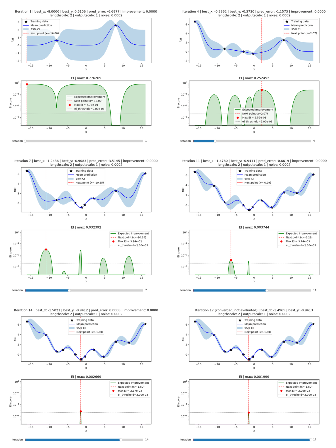
The blue band is the GP’s 95 % confidence interval. It is wide wherever the objective has not been evaluated and pinches shut around each training point, so watching it narrow around x = -1.5 is watching the surrogate become certain. Below it, the EI curve peaks where the next evaluation is most worth spending, and collapses towards ei_threshold as that certainty grows.

It converges after 17 iterations via ei_threshold, at best_x = -1.4965, best_y = -0.9413. The true minimum sits at x = -1.49593, so the run lands within 5.5e-4 of it after only 18 objective evaluations: the 2 initial points plus one per evaluated iteration. The 17th iteration triggered convergence and was never evaluated.

Fixed hyperparameters (without_training) are why each title’s second line stays constant across the frames; with_training would show them retuned every iteration.

Step 5: check that it converged

The slider shows what the surrogate believed at each step. The metrics figure shows whether the run as a whole got anywhere:

run.plot_metrics()

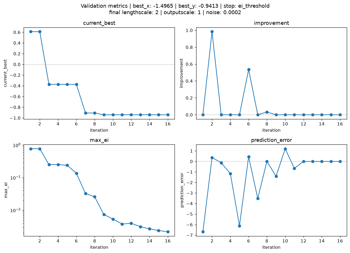
Four panels, one per metric, for the same run as the animation above:

current_best

The lowest objective value found so far. It steps down and then flattens, which is the run finding the minimum and then confirming it.

improvement

How much each evaluation lowered current_best. It spikes early, then sits at zero once the optimiser is refining rather than discovering. Flat improvement while max_ei is still high means the search is exploring, not finished.

max_ei

The convergence signal, on a log axis. It falls by three orders of magnitude and the run stops when it crosses ei_threshold. A run that has not converged shows this line still comfortably above the threshold.

prediction_error

predicted_y - new_y: how wrong the surrogate was about the point it just chose. Large and swinging either side of zero early on, then settling towards zero as the surrogate learns the objective.

One panel per metric rather than one shared axes: the four have unrelated units and ranges, so overlaying them flattens all but the largest into a line along zero. max_ei is the only one that can take a log axis, since prediction_error is signed and improvement is frequently exactly zero. Pass log_scale=False to make that panel linear too.

Step 6: the reproducibility record (MRR)

Because run_dir was given, the run created a timestamped folder under results/ holding the five MRR artifacts:

• config.json: every parameter used, written at the start of the run

• manifest.json: a SHA-256 checksum of the inputs

• meta.json: environment, covering package name, version, and repository, git commit, Python/library versions, platform, timestamps, and output summary

• run.log: a human-readable, per-iteration audit trail, ending with a summary line giving best_x/best_y. That line is the quickest way to read off the identified minimum without opening results.h5 or inspecting the run.run() return value

• results.h5: self-describing HDF5, where configuration is stored as attributes alongside the data, so the file can be understood on its own

To browse results.h5 without writing code, the H5Web VS Code extension opens HDF5 files directly in the editor, showing groups, attributes, and plots of any dataset.

If the run raises partway through, meta.json and results.h5 are still written as a best-effort checkpoint covering every iteration completed before the failure (stop_reason="crashed"), and run.log ends with an error line instead of the summary line.

Revisiting a saved run

Both figures can be rebuilt from a run directory alone, with no OptimisationRun object, so a past run can be revisited at any later time. load_metrics draws the validation metrics:

from pathlib import Path

from actgpr.plotting import load_metrics

run_dir = sorted(Path("results").iterdir())[-1]   # newest run
load_metrics(run_dir)

and load_iterations opens the same interactive slider as run.plot_iterations():

from actgpr.plotting import load_iterations

slider = load_iterations(run_dir)

Assign the slider to a variable that outlives the call. Matplotlib keeps only a weak reference to it, so a slider left unassigned is garbage collected: it is still drawn, but silently stops responding to drags.

The slider needs the run to have kept snapshots (the default). It raises RuntimeError for a run executed with store_snapshots=False, since the per-iteration GP arrays were never written. load_metrics works either way, since the validation metrics are always recorded.

For a custom analysis, read the same series directly:

import h5py

with h5py.File(run_dir / "results.h5") as f:
    iteration = f["history/iteration"][:]
    prediction_error = f["history/prediction_error"][:]
    improvement = f["history/improvement"][:]

Parameter reference

with_training and without_training share the same core parameters and differ only in how the GP hyperparameters are handled.

Shared parameters

Parameter	Meaning
objective	The blackbox to minimise: an ObjectiveFn or any object with evaluate(x1, ..., xd) -> float.
surrogate	The GP surrogate backend. Pass a fresh GPyTorchSurrogate(), since it holds fitted state internally, so do not reuse one across runs.
search_bounds	One closed interval (lo, hi) per input, e.g. [(-2.0, 2.0), (0.0, 5.0)]. Their number is the number of inputs. A single (lo, hi) means one input. The blackbox is never evaluated outside them.
initial_train_x	Points where the search starts, one row per point with one coordinate per input, e.g. [[0.0, 1.0], [2.0, 3.0]]. With one input a flat list such as [-3.0, 5.0] is accepted. The first surrogate is fitted to these before the loop runs. With one input, a common choice is the two search_bounds endpoints.
max_iterations	Budget cap: the maximum number of active optimisation iterations (GPR fit cycles), not individual blackbox evaluations.
ei_threshold	Convergence threshold: the run stops early once the best achievable Expected Improvement drops below this value.
n_candidates (default 500)	Number of candidate points the acquisition function scores in each of its two stages every iteration: an evenly spaced grid with one input, a seeded Sobol sample with more. Raise it for many inputs.
noise (default 1e-4)	Starting observation noise variance for the GP likelihood. In with_training it is only a starting point, since Adam tunes it further alongside lengthscale and outputscale. In without_training it stays fixed at this value for the whole run.
store_snapshots (default True)	Keeps each iteration’s full GP/EI arrays (in memory and under results.h5’s iterations/ group) so plot_iterations() can browse them afterward. Set False to omit them, since they are the bulk of results.h5’s size. The prediction_error/improvement history used by load_metrics() is recorded either way.
run_dir (default None)	If given, writes the MRR record (see Step 6) to a timestamped folder under this path. If None, nothing is written to disk.

with_training only

Parameter	Meaning
training_iter (default 50)	Number of Adam optimisation steps run per surrogate fit, tuning lengthscale, outputscale, and noise to maximise the marginal log likelihood.

without_training only

Parameter	Meaning
lengthscale (default 1.0)	Fixed RBF kernel lengthscale, never tuned. One value used for every input, or a list with one value per input.
outputscale (default 1.0)	Fixed kernel signal variance, never tuned.

Plotting reference

Two figures, each reachable two ways. That is four entry points in total, and there is nothing else to learn.

The prefix says where the data comes from. plot_ draws from the run object you are still holding, so those two are methods on OptimisationRun. load_ takes the path to a run’s log directory, reads its results.h5, and draws the same figure, so those two are functions imported from actgpr.plotting.

	The surrogate itself	Validation metrics
From the run	run.plot_iterations()	run.plot_metrics()
From the logs	load_iterations(run_dir)	load_metrics(run_dir)

The bottom row needs run_dir to have been set, since it reads results.h5; the methods work either way. run.run_dir holds the timestamped directory the run wrote to, so the two functions also work on a run you just finished, not only on one from last month.

Use	What it draws
run.plot_iterations()	Start here. An interactive slider over every iteration of a finished run: the GP fit on top, the EI landscape below. Watching the band narrow around the minimum is the clearest picture of what the algorithm did.
run.plot_metrics()	The whole run as one figure, four panels: current_best, improvement, max_ei (log-scaled), and prediction_error against iteration. Use it to judge convergence at a glance.
load_iterations(run_dir)	The slider again, read back from a run’s logs. Keep the returned Slider in a variable or matplotlib will collect it and it will stop responding.
load_metrics(run_dir)	The four panels again, read back from a run’s logs.

Each pair draws the identical figure, so which one to reach for depends solely on what you still have to hand.

All four open their window by calling plt.show() for you. That is fine for a single figure, but plt.show() opens every figure that exists, not just the one you last built, so two calls in a row open the first window a second time. Pass show=False to build a figure without opening it, then call plt.show() once at the end to open everything together:

import matplotlib.pyplot as plt

slider = load_iterations(run_dir, show=False)
load_metrics(run_dir, show=False)

plt.show()   # once, for both

Both windows are titled (actgpr: iterations (GP fit and EI) and actgpr: validation metrics), since matplotlib opens them at the same position and one lands on top of the other.

All four also take log_scale=False: on the slider it makes the EI panel linear, on the metrics figure it makes the max_ei panel linear.

Log is the default because EI falls by orders of magnitude as a run converges, so on a linear axis it sits flat against zero and its decay towards ei_threshold is invisible. The other three metrics stay linear either way, since prediction_error is signed and improvement is frequently exactly zero, neither of which a log axis can display.

What each raises

The iteration figure needs the per-iteration snapshots of a one-input run; the metrics figure needs only the per-iteration series, which are always recorded. So the two fail in different situations, each with a message naming the actual cause:

Situation	What you get
run_dir holds no results.h5	FileNotFoundError, from either load_ function
The run used store_snapshots=False	RuntimeError from load_iterations/plot_iterations, telling you to re-run with store_snapshots=True. load_metrics/plot_metrics work normally
run() has not been called yet	RuntimeError from either method, telling you to call run() first
The run has more than one input	ValueError from load_iterations/plot_iterations, since the surrogate cannot be drawn as a curve. load_metrics/plot_metrics work normally

Where to go next

• The API reference documents every class and function.

• The README’s vocabulary section defines every term used in this package.